目录
Resource Info Paper http://arxiv.org/abs/2509.07558 Code & Data https://github.com/zerolllin/Delta-L-Normalization Public arXiv Date 2025.09.22
Summary Overview
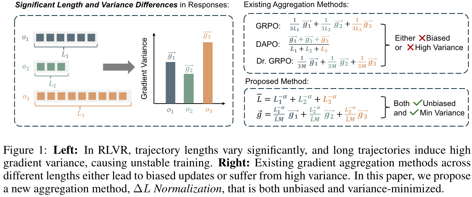
Although previous methods such as GRPO, DAPO, and Dr. GRPO introduce different loss normalization terms to address this issue, they either produce biased estimates or still suffer from high gradient variance. By analyzing the effect of varying lengths on policy loss both theoretically and empirically, we reformulate the problem as finding a minimum-variance unbiased estimator. Our proposed not only provides an unbiased estimate of the true policy loss but also minimizes gradient variance in theory.
Main Content
GRPO applies a sample-level normalization, dividing each sample-level loss by its response length; while DAPO uses a batch-level approach, normalizing the total loss by the sum of response lengths in the batch. In addition, because such length-dependent factors deviate from standard reinforcement learning theory. Dr. GRPO, in contrast, avoids any length-dependent factor and normalizes the gradient with a fixed constant.
There is a lack of analysis on how they influence the statistical properties of gradient estimation in RLVR, with gradient variance being particularly important because high variance leads to inefficient training and even model collapse.
(1) The aggregation startegies in GRPO and DAPO introduce length-dependent bias in estimating the true policy gradient. As response lengths increase, their parameter updates shrink in gradient norm, slowing convergence. (2) The aggregation strategies in DAPO and Dr. GRPO lead means greater relative noise for the same gradient norm, resulting in less stable training.
the variance of the unnormalized gradient grows approximately proportionally to the response length.
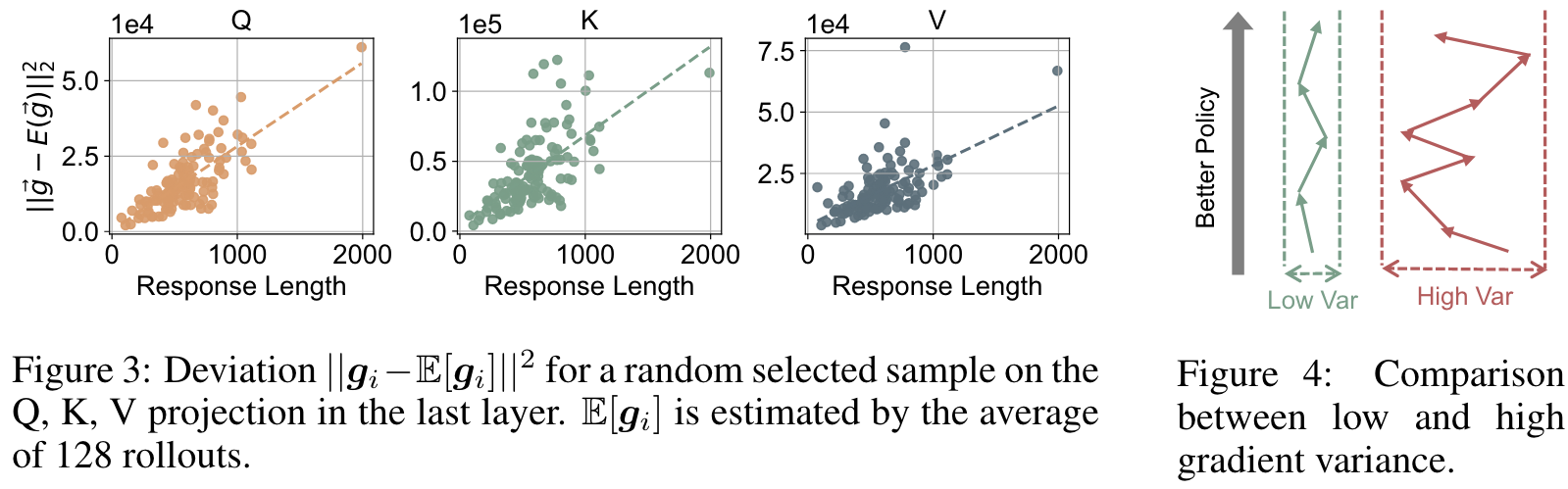
Consider . We approximate this as , by ignoring covariance between individual token-level gradients. Assuming each token-level term contributes approximately a constant variance , we thus have . This approximation indicates that samples with longer responses inherently exhibit higher gradient variance due to increased randomness, and the gradient variance grows proportionally with response length.
GRPO and DAPO introduce length-dependent coefficients determined by the response lengths , which results in a issue.
Rethink loss normalization in RLVR
Existing aggregation methods introduce either bias or excessive variance. We therefore ask: The answer is yes. We observe that this problem can be naturally reformulated within the framework of minimum variance unbiased estimation in statistics. Specifically, we treat the gradients obtained from responses of different lengths as independent observations of the same underlying variable (the ground-truth policy gradient), each with its own variance. Our objective is then to construct a new unbiased estimator by optimally combining these observations so that the resulting variance is minimized. Formally, we define the problem as follows.
Problem Definition. Given a set of independent sample-level gradient estimators satisfying and , where denotes the length associated with sample and is a constant scalar, the objective is to determine coefficients in the linear combination , such that for a given , while minimizing the variance .
Noting that the unbiasedness constraint is equivalent to and, by independence, the variance satisfies , the problem reduces to a convex quadratic program with a single linear constraint. Solving with the Lagrange multiplier method yields the unique minimizer: .
In practice, we find it is beneficial to introduce a hyperparameter to the normalization factor, which gives the following normalization weights:
The parameter provides a tradeoff between variance reduction and utilization of long responses. While longer responses tend to introduce higher variance, sometimes they also carry richer learning signals. Choosing allows these signals to contribute more effectively, at the cost of increased gradient variance. We name this method , as it is specially designed to match the dynamic length nature in RLVR. It has four key properites:
- Unbiasedness: For any , is unbiased since , ensuring . This preserves theoretical consistency with vanilla reinforcement learning.
- Minimum Variance: Choosing achieves the minimum possible variance under the unbiasedness constraint. Under the assumptions, this is the unique solution when loss aggregation is a linear, unbiased combination.
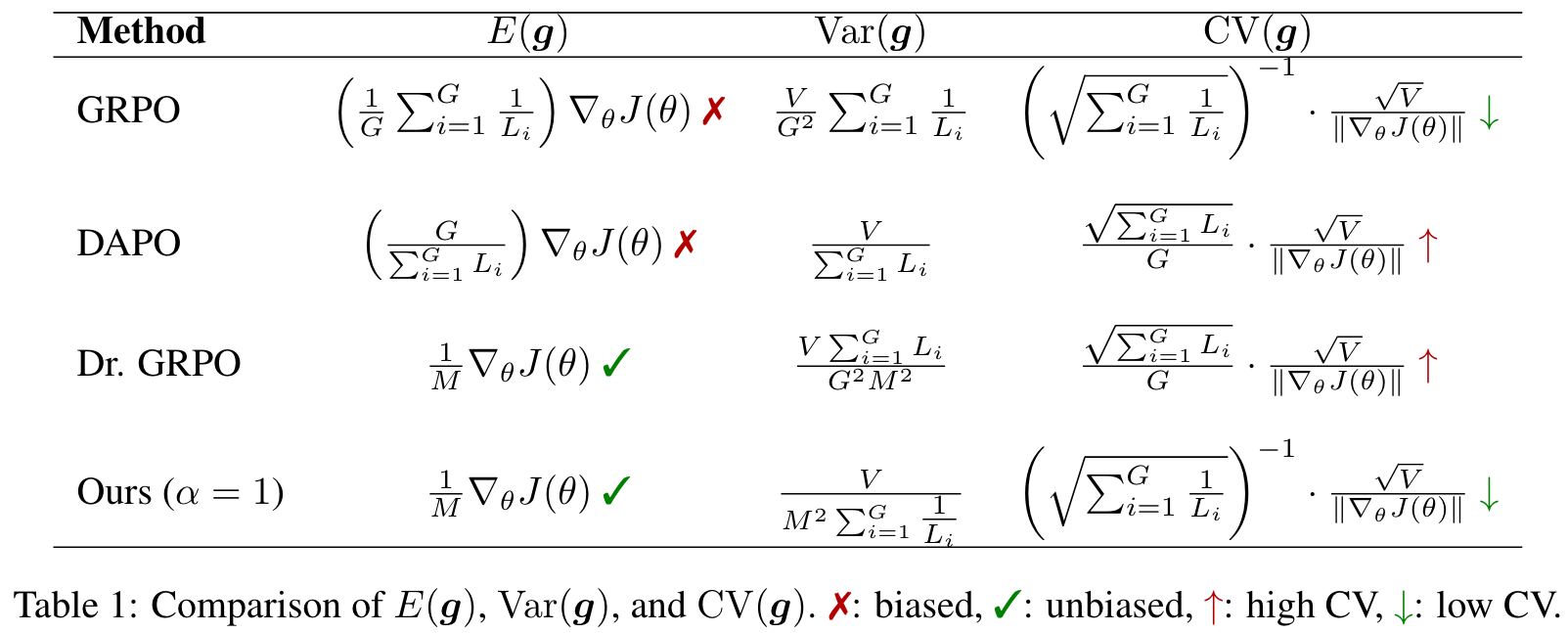
- Controlled Coefficient of Variation (CV): We can show
Thus, guarantees lower CV than DAPO and Dr.GRPO, while matching GRPO at . When , variance increases slightly, but long responses contribute more effectively.
- Transition to Dr.GRPO: Setting recovers the aggregation method introduced in Dr.GRPO, making it a special case of .
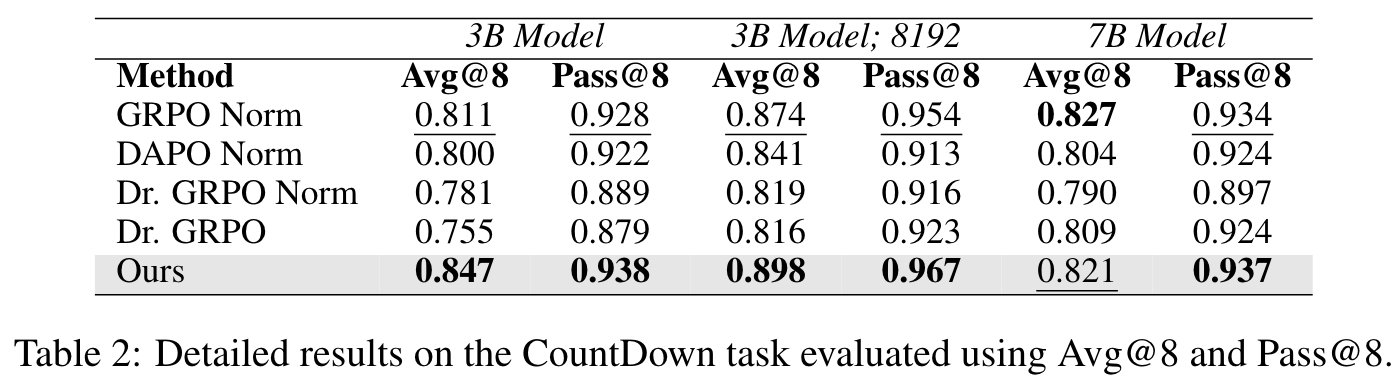
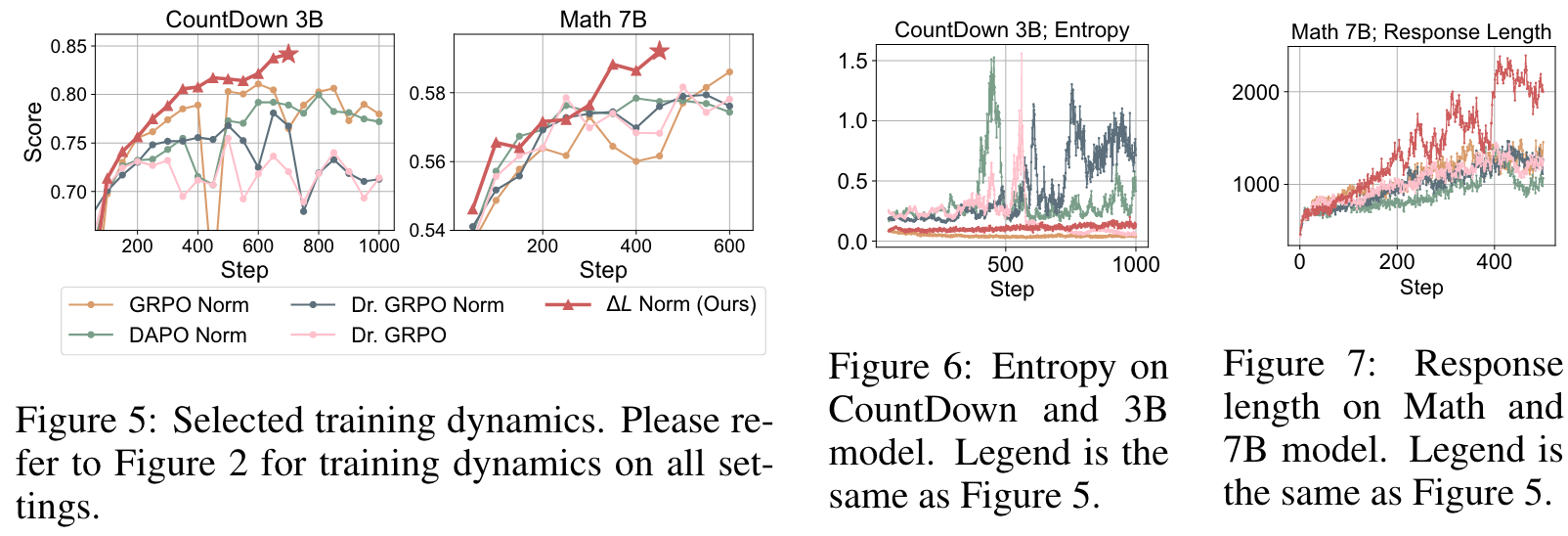
These properties make highly valuable for RLVR training. The unbiasedness property ensures consistency with standard reinforcement learning theory, preventing unexpected slowdowns caused by biased gradient estimates. Variance reduction further stabilizes training and accelerates convergence. In practice, we find that, setting , which minimizes the variance, is a universal good choice. further increase the performance in Math, which might be due to the fact that the long response in Math task should be better utilized.
🤖
-
论文的创新之处与独特性:
- 创新点:
- 提出了一个新的损失聚合方法——∆L Normalization,专门针对强化学习中动态生成长度的挑战。
- 通过理论和实验分析,∆L Normalization被证明能够提供无偏估计并最小化梯度方差,从而解决现有方法(如GRPO、DAPO和Dr. GRPO)中的偏差或高梯度方差问题。
- 设计了一个简单但有效的长度归一化公式,并引入了可调参数α以平衡长响应的贡献与梯度方差。
- 关键学习点:
- RLVR的训练中,响应长度的显著变化会导致梯度方差的线性增长,影响模型稳定性。
- 通过最小方差无偏估计框架,可以优化梯度聚合方法,从而提高训练稳定性和模型性能。
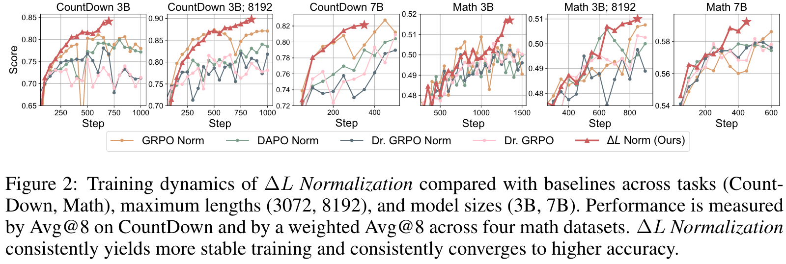
- ∆L Normalization在多个任务和模型规模上均表现出一致的优越性。
- 创新点:
-
论文中存在的问题及改进建议:
- 问题:
- 参数α的选择对任务性能影响较大,但论文中对如何选择α的指导有限,尤其是针对不同任务的具体调整策略。
- 实验部分虽然涵盖了多个任务和模型规模,但对更广泛的应用场景(例如非语言任务或多模态任务)缺乏验证。
- 对于其他可能的辅助优化技术(如动态采样和惩罚机制),∆L Normalization的组合效果未充分探索。
- 改进建议:
- 提供更详细的α选择策略,例如通过任务特性评估或自动调参方法优化α。
- 扩展实验范围,验证∆L Normalization在非语言任务或多模态任务中的适用性。
- 探讨与其他优化技术(如动态采样或惩罚机制)的协同作用,并开发更全面的训练框架。
- 问题:
-
基于论文的内容和研究结果,提出的创新点或研究路径:
- 创新点1:结合∆L Normalization与自动调参技术(如贝叶斯优化或强化学习)以动态调整α。
- 创新点2:探索∆L Normalization在多模态任务(例如视觉-语言任务)中的应用,并研究其对不同模态数据的梯度方差影响。
- 创新点3:开发一个统一的RLVR优化框架,将∆L Normalization与动态采样、惩罚机制以及其他先进技术整合,以应对更复杂的任务。
-
为新的研究路径制定的研究方案:
- 研究方案1:动态调参的∆L Normalization
- 目标:通过自动调参技术优化α值,以适应不同任务的动态特性。
- 研究方法:
- 使用贝叶斯优化或强化学习算法,动态调整训练过程中α的值。
- 在多个任务(如数学推理、语言生成)中验证动态调参的效果。
- 比较动态调参与固定α值的性能差异。
- 步骤:
- 定义优化目标(如梯度方差最小化或模型准确率最大化)。
- 设计动态调参算法,将任务特性(如响应长度分布)作为输入。
- 实验验证,并记录训练动态和最终性能。
- 期望成果:验证动态调参的有效性,并提供通用的α优化策略。
- 研究方案2:∆L Normalization在多模态任务中的应用
- 目标:探索∆L Normalization在多模态任务中的适用性,并优化跨模态的数据处理。
- 研究方法:
- 选择多模态任务(如视觉问答或图像生成)进行实验。
- 分析不同模态数据的梯度方差特性,并调整∆L Normalization公式。
- 设计实验验证其对模型稳定性和性能的提升。
- 步骤:
- 收集多模态数据集,并设计适合RLVR的训练任务。
- 改进∆L Normalization公式,使其适应多模态数据的特性。
- 进行对比实验,分析∆L Normalization的效果。
- 期望成果:证明∆L Normalization在多模态任务中的适用性,并提出优化建议。
- 研究方案3:统一的RLVR优化框架
- 目标:开发一个整合∆L Normalization、动态采样和惩罚机制的统一优化框架。
- 研究方法:
- 将∆L Normalization与动态采样和惩罚机制结合,设计统一的训练流程。
- 在不同任务中评估框架的性能,并与单独使用∆L Normalization的方法进行对比。
- 步骤:
- 研究动态采样和惩罚机制的理论基础,并分析其与∆L Normalization的协同作用。
- 设计实验,验证整合框架的性能。
- 提出改进建议,并优化框架设计。
- 期望成果:开发一个更强大的RLVR优化框架,适用于复杂任务和大规模模型。
- 研究方案1:动态调参的∆L Normalization
Others
本文作者:Geaming
本文链接:
版权声明:本博客所有文章除特别声明外,均采用 BY-NC-SA 许可协议。转载请注明出处!